

result

result


PREVIOUS
NEXT
Follow Us
All content Copyright 2023 Fixed Income Insights. All rights reserved.


Executive Summary
Every investment in the MBS market is “long duration/short volatility.” A proxy for MBS is to buy an Agency bullet and short/sell options to earn additional income. The level of volatility is the price of the options, and therefore, it determines how much income is earned. However, volatility in this context is not directly observable; rather it is “implied” by the price of the option in relation to its strike price and tenor. This article will explain how volatility is used to price MBS assets and what the current level of volatility may mean for the sector going forward.
The basic concept is this: All taxable fixed income decisions of risk and reward come down to these three factors: 1. duration, 2. credit, and 3. optionality. Those are the levers investors can pull to make money and hedge risk. Sometimes, exogenous factors such as central bank involvement and other “liquidity” factors play a role, but these three are the bedrock of fixed income investing. For this article, we will assume little to no credit risk among the various examples and we will concentrate as often as possible on duration-neutral choices in order to isolate the focus factor: volatility exposure.
The data in Table 1 highlight this trade-off around volatility/yield very well. It is a simple list of four assets, all with practically the same OAD, sometimes known as effective duration. The list is purposely made in the order of volatility duration, from lowest to highest.
Table 1: Higher Volatility Exposure Should Render Higher Yield/Spread

The list is based on the 5yr UST note, because that is a typical duration point that resides in almost all fixed income mandates. The list was then expanded to include various levels of first, liquidity preference, and then increasing exposure to optionality/volatility. The list is very short at this stage for illustrative purposes and will be expanded with additional information later.
The second item, the 5yr bullet, has a yield very close to that of the 5yr UST note, but not exactly the same. This particular bullet is a 5yr FHLB auction bond, so there is a small liquidity preference mismatch with the UST note. The next item is a 15yr 2.5 passthru. It also has a higher yield, but that is not due to any liquidity preference. That is due to the fact that the 15yr passthru has some, but not much, exposure to optionality/volatility. Therefore, the volatility duration is positive, although rather small compared to other assets on the larger list shown below.
The fourth and final item on this abbreviated list is a 30yr 4.5 MBS passthru. This bond has quite a bit more exposure to optionality/volatility, as shown on the far right of the analysis. Therefore, it also has a much higher yield and much wider z-spread than the other assets in order to compensate the investor for the greater optionality.
This leads to the question, if the volatility is implied from the model, what is the option that is being priced to produce the implied volatility? For a callable bond (agency or corporate), the answer is straightforward. The issuer has the option to call the bond and pays for that option by financing at a higher yield to the investor. That sort of option is priced with a binomial lattice or “tree” that prices each potential call in time on its own merit. The volatility implied in the price of the (call) option explains how wide a binomial lattice or “tree” can get from one potential call date to another. In the picture of the binomial lattice on the next page, in any case that the price of the bond goes above par, the bond is called. The wider the lattice, the more times the bond will price above par therefore, the higher the probability the bond will be called. This leads to a wider spread for the bond due to the higher price of the imbedded option.
Figure 1: Picture of Binomial Lattice for a Callable Bond
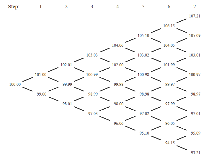
Source: Macroption.com
For a mortgage bond, the price of the prepayment option is “free” to the issuer, i.e. the borrower. However, collectively, all mortgage borrowers have to pay a rate above that of an Agency bullet to compensate investors for the possibility that any one or a number of loans will be called at any given time. But the options models do not look to the borrower to price the option. Rather, they look to the “swaptions markets.”
The reason for this market convention for pricing MBS options is the traditional GSE business model. The GSEs now are in the business of guaranteeing principal and interest payments on mortgage-backed securities to effectively eliminate the credit risk to MBS security holders. But before 2006, the GSEs also had an additional important function: market buyer of last resort of MBS paper.
This second prong of the traditional GSE business model produced the market conventions of “LIBOR OAS and using the “swaptions” markets to price mortgage securities that models still use today. To put it very simply, the GSEs, as the MBS buyers of last resort, would issue callable agencies and swap out that exposure in the swaptions markets to fund at LIBOR less some spread. They would use those funds to purchase MBS and then swap out those cash flows at LIBOR plus some spread. Given that callable agencies price on the lattice explained above and MBS price using a method called a Monte Carlo simulation meant that the transactions did not produce perfect hedges. However, in the aggregate, the GSEs normally disclosed that their “duration gaps” between assets and liabilities were very minimal during most reporting periods.
Obviously, the portion of the GSE business models regarding extraordinary MBS purchases went away as a result of policy changes after the Great Financial Crisis in 2008/2009. (The GSEs controlled as much as 1/3 of all MBS securities on balance sheet, in addition to guaranteeing the principal and interest payments of all of them, at the peak.) However, the pricing conventions of OAS and using the swaptions markets have survived.
The most common form of this model today is an odd mix of using Treasuries as the discount curve and LIBOR swaptions for the OAS model. With the upcoming transition away from LIBOR to SOFR, it is likely that market participants in the future will use the SOFR discount curve and SOFR swaptions. However, we will use TOAS and LIBOR swaptions for our examples given the rich availability of historical data.
A swaption is a contract that allows the owner to either start or cancel an interest rate swap, depending on the desired direction of the trade. The pricing of that option depends on a host of factors, not the least of which is volatility. Or, to put it more precisely, the volatility imbedded or “implied” in the contract is a result of the other inputs to the model, such as the tenor of the swap, the time to expiration of the option, and the “strike price” or interest rate on the fixed-rate leg of the swap. A higher volatility means that the option is more expensive for the party that is buying the right to execute the swap in the future.
In reality, very few MBS players actually use the swaptions markets anymore. Large banks and dealers do sometimes, as do hedge funds. But most MBS players are much more buy-and-hold and do not execute swaptions on the funding side of the market, like the GSEs did, in great size. However, the conventions have held on, and most OAS models still use swaptions volatilities to run the Monte Carlo simulations for the OAS models.
With this long explanation as the background, we now make the turn toward application. We are going to look at LIBOR swaption volatilities in two ways: 1. The current “volatility surface” and 2. One point on the vol surface historically.
Figure 2: Implied Volatility Surface is a 3D Function

As noted above, a swaption is an option to start or cancel an interest rate swap within some other time frame. So the graph of volatilities is actually a three-dimensional picture with three axes, instead of just two axes for a typical line graph such as a scatter-plot or time series. The first axis in this picture is the option expiration, or for how long is the option outstanding. The second axis is the tenor of the swap: one-year, five-year, 10-year, etc. The third axis represents the levels of volatility implied by the price of the various options in the chart.
It should be noted that the levels shown here are “normalized” volatility. These are not the actual numbers that come out of the model. Those are known as “percent” or “Black” vol, named after the mathematician/economist Fischer Black who, along with Myron Scholes, pioneered option pricing models. But in fixed income, it is important to normalize the level of volatility to interest rates by using basis points. For example, a 25 bps move in a 2.00% rate market will be twice the percent move as in a 4.00% rate market. Therefore, normalizing to basis points allows for better comparisons over time.
An astute observer may note that the current volatility surface displayed in Figure 2 may look “backwards.” After all, options with longer tenors should be priced higher, and the option premiums ARE higher for the longer tenors. However, this is not a chart of options prices – rather it is a chart of one of the implied (i.e. not visible) inputs: annualized volatility. With so much uncertainty surrounding the Fed during the next two years, it is no wonder that volatility for short-expiry options on shorter-tenor swaps is so high.
A concrete example may help. One of the more oft-quoted swaptions is the one-month-into-10-year contract. This may be a contract used by a mortgage pipeline hedger. It allows the user to determine in one month what will be the duration hedging costs of a mortgage loan taken out today to settle in one month, and the swaption premium is the cost of this ability to “pre-hedge.” The advantage of this example is that it is related to the MBS market.
The rest of the volatility surface is, however, less related to the MBS market than it used to be, because it is less directly tied into the funding of MBS through the GSEs. In the past, if Fannie or Freddie would issue a 5-year/no-call-2-year Global deal, for example, they could execute a 2-year-into-3-year swaption to hedge that risk and convert it to floating. (That is, they would “buy” the option to start or cancel a three year swap at the same date that they would be long the call option on the bond, with the same tenor as the remainder of the bond.) That being said, the FHLB and FFCB, among others, are still active in the swaptions markets, and the models still use swaption vols to build the volatility surface in the models for the Monte Carlo simulations for MBS.
Using our one-month-into-10-year example, we can observe how swaption volatility changes over time. Of course, vol is not constant, and neither is the shape of the vol surface. But it is beyond our already in-depth analysis to present a study of ALL potential swaption vols. So we will allow the implied volatility in this one contract to be the main example.
Figure 3: Implied Vol Is Still Slightly Above or Well Above Average, Depending on Perspective
The current level of implied volatility in the swaptions market is above “average” but by a lesser amount than last October. If that looks familiar, it should. MBS spreads were also at their recent wides last October. The relationship between implied vol and MBS spreads is, therefore, not a coincidence. Due to the reliance of the market – perhaps misplaced at this juncture – on the OAS framework of relative value, it makes sense that the MBS market and implied volatility would be linked. In fact, one can clearly see in Figure 3 the GFC in 2008/2009, “taper tantrum” in 2013, the onset of the Covid-19 restrictions in early 2020 and the ugly response by the MBS market in 2022 as the Fed pulled back support. One can also clearly see how the Fed suppressed vol during much of 2014-2018 and for a brief time in 2020-2021, this latter period despite record levels of refi activity in MBS. And that was probably why the “unwind” of Fed support was so painful in terms of performance in 2022.
It is time to land the plane with this question: What does the current state of the swaptions markets mean for MBS investors? We will leave aside potentially the trickiest aspect of this, LIBOR transition, and simply assume that there will be some reasonable facsimile created with SOFR in the future. In fact, the CME group is working on this very mandate.
The real question is how “cheap” are MBS through the lens of implied volatility and how will potential changes in vol affect MBS performance? A review of Figure 3 reveals two main points. First, implied volatility, despite the drop to start the year, is now moving higher again as a result of the bank failure narrative. It is now almost three standard deviations above the 10yr average that includes taper tantrum. Furthermore, implied volatility is almost 1.5 standard deviations above its average since 2005, and that includes the Great Financial Crisis. Second, the size of a standard deviation for the 18yr lookback is 34 bps and it is 21 bps for the 10yr lookback. Therefore, we split the difference and ran a longer list of bonds in Table 2 below by shifting the volatility surface up and down 25 basis points to see the impact on TRR performance, assuming constant-OAS pricing at the horizon.
Table 2: Longer List of Mortgage Asset Reactions to Changes in Implied Volatility
This list contains the 15yr and 30yr coupon stack in MBS collateral and the same agency bullet found in Table 1 above. The trick with this sort of analysis is to limit the number of line items to something useful, so we are allowing the generic coupon stack to represent all MBS.
There is an output in YieldBook called “volatility duration,” and it displays the exposure of the bond to a one bp change in implied volatility. That typically produces a very small number, so we gross it up to 100 bps to display a useful number. The list is then sorted by that adjusted volatility duration, from lowest to highest. The results of our volatility shocks are on the right. The final two columns, which are color-coded from lowest (red) to highest (green) are the difference in TRR between that scenario and the “base case.” In other words, these two calculations isolate the effects of an increase and decrease, respectively, in implied volatility by 25 basis points.
Generally, the sign for volatility duration is the same as for effective duration: a bond with a positive volatility duration should experience positive TRR performance if volatility falls.
In addition to these exceptions, there are two general patterns we see in these examples:
- The longest OAD bonds tend to have the most exposure to changes in implied volatility, even if they are at deep discounts. Another way to say this, and this is very important to grasp, is that convexity and implied volatility exposure are NOT the same thing. Convexity is the rate of change in duration. Convexity is technically not a surrogate calculation for volatility exposure. A very long bond can have a great deal of exposure to changes in implied volatility due to it being outstanding for longer, but it may also have positive or near positive convexity.
- Bond structure drives vol duration more than anything. The 15yr sector has less vol exposure, even for bonds that have the same OAD as higher-coupon 30yr counterparts. Even though they are not displayed here, the same is true of front-pay CMOs: they tend to have very little exposure to changes in volatility.
In summary, implied volatility is an important concept for MBS investors to grasp, even as the lack of observation of this variable makes it a bit intimidating. For those who prefer option Greek terminology, these translations for fixed-income options may be helpful:
- Duration = delta, the first derivative of the price/yield function
- Convexity = gamma, the second derivative of the price/yield function
- Volatility = vega, the first derivative of the price/volatility function